

Microsoft Excel is one of the most convenient and popular spreadsheet apps. Since many people do their reporting exactly in Excel. The program has many handy tools to make this task as easy as possible.
If you need to process data that is related to dates, Excel has a special tool that you can use to add months to your dates. This is especially useful if you need to compile a monthly report in such a way that you can then easily transfer it to the next month. The best way to add months to your dates is to use the EDATE formula.
How to edit date in Microsoft Excel
If you need to constantly update the date and add months to it, you can use a special function for this. Of course, you can do this manually, but that way it takes quite a lot of time. Also if you need today’s date, I would suggest doing it with the [Ctrl + ;] key combination.
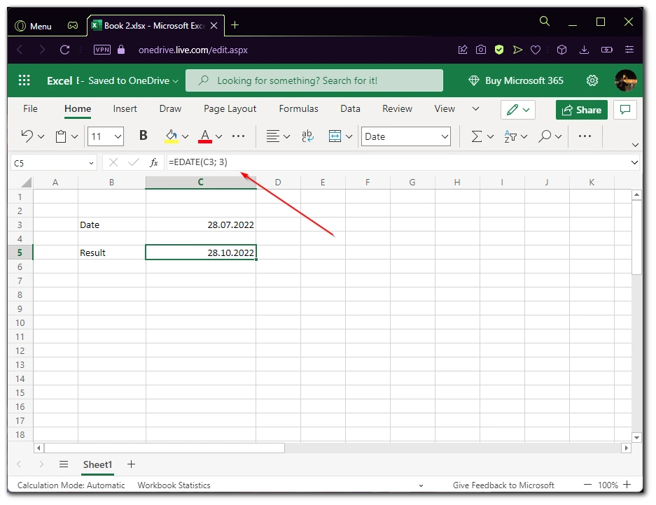
However, if you want to do a report every month on the same day, you can use the function =EDATE(start date, number of months) to add the month to the date you want. The most convenient way is to use it with a special cell where the start date will be written. To do this:
- Enter the start date in the desired cell.
- Then, in the cell where the result date will be shown, write the following function
=EDATE(start date; number of months to be added). In the example below it looks like=EDATE(C3; 3). This function works for adding 3 months.
- You also need to make sure that the cell with the final result is formatted correctly, otherwise, it will just show a numeric value instead of the date. To do this, use CTRL + 1 and select date formatting.
The main thing is to make sure that the cells are formatted correctly. This is usually where a lot of people have problems.
How you can format date in Microsoft Excel
Also, if you go into the option to format the cells, here you can choose different displays for your date. This can be useful in various cases. For example, if you are making a table for Europeans or for Americans, the date format should be different. Also, for example, you don’t need to put the year if you have a table made for a specific year and only need days and months.
To go to the format option, select the desired date cell and press [CTRL + 1]. When you go to the Date tab in the formatting option. Here in the list, you can select the options you want from the examples and in the upper field, you will see how your date will be displayed.
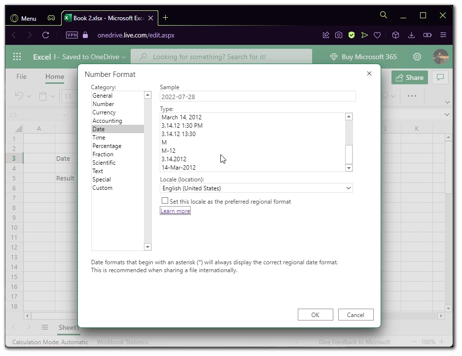
You also need to select the location so that Excel will automatically determine your preferred format and translation of the month name. You should also remember that you can add to the date the exact time when you entered it in the cell.
How to add or remove days from a date in Excel
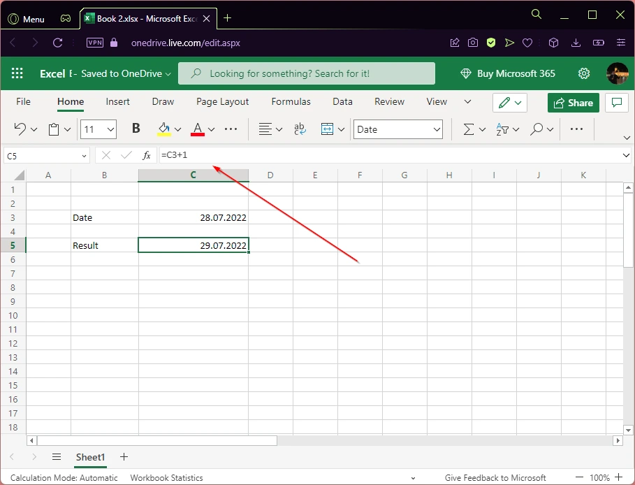
If you just need to add a couple of days, it’s a lot easier to do. So of course you can also add months if you just add more than 30 days. To do this you need to:
- Enter the starting date in one cell.
- In the second cell, enter the formula
= [cell with starting date] + [number of days you want to add].
As you can see, a simple addition formula is used here. Again, you need to make sure that all cells are formatted correctly. If you made a mistake with the formatting, you can look at the history of changes and return everything as it was.
Read also:
- How to get currency exchange rates in Microsoft Excel
- How to switch the X and Y-axis in Microsoft Excel
- How to use the SUBSTITUTE function in Microsoft Excel
How to change the colors in the table
In my work, I quite often encounter different tables. To make them palatable, I have to devote some time to formatting. You should align the text, bold or underline the necessary elements and apply the right font.
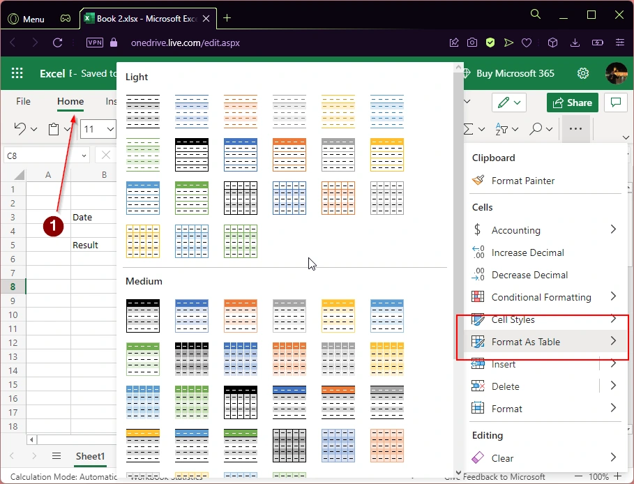
However, in my experience, one of the best solutions to make your table unique and memorable is to add colors to it. In Excel, there is a feature that allows you to add alternative colors to your spreadsheet. This means that the icons will alternately change in 2 different colors. It is also possible to make smooth transitions for larger or smaller numbers. This will help you highlight the information you want and make the table as personalized as possible.
To do this you need to select the area to which you want to apply this feature and then select the tab Home in the toolbar. Then go to Format as Table to add alternative colors. You can also use different options from Conditional Formatting or Cell Styles.
I can advise you to apply neutral colors to any important table to make it more pleasing. And don’t forget to add Headers after choosing a color.
