

One commonly used formatting element in Microsoft Excel is the checkmark symbol, which can indicate completion, approval, or any other appropriate status in an Excel spreadsheet. However, I was stumped the first time I needed to put a checkmark in a cell. It’s hard to find that symbol in Excel if you don’t know where to look. I have found several ways to help me check and close tasks in Microsoft Excel.
How to insert check marks in Microsoft Excel using the Symbol button
One straightforward way to insert a checkmark symbol in Excel is by using the “Symbol” command. To do this, you need the following:
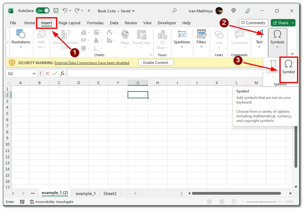
- Select the cell where you want to insert the check mark. Then, navigate to the “Insert” tab in the Excel ribbon, and click on the “Symbol” button in the “Symbols” group.
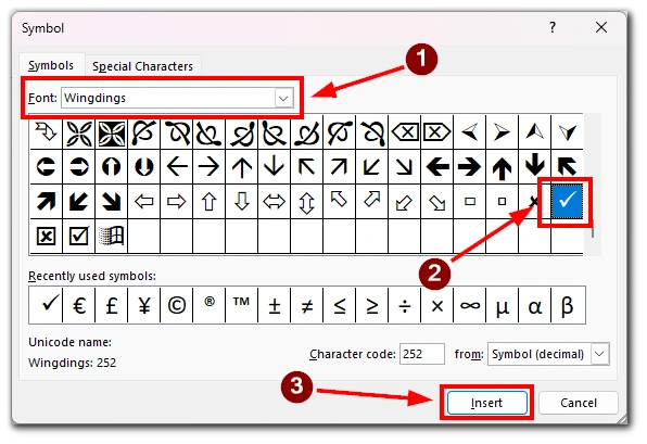
- A dialog box will appear, displaying various symbols and special characters. Select “Wingdings” in the Font field. Locate the check mark symbol from the available options or use the search functionality to find it quickly. Once you find the check mark symbol, select it and click the “Insert” button.
The symbol will be inserted into the selected cell, and you can resize or reposition it as needed. This method is useful when you only need to insert a few check marks manually, but it can become time-consuming if you have many cells to update.
How to insert check marks in Microsoft Excel utilizing AutoCorrect
Excel’s AutoCorrect feature provides another efficient way to insert check marks in your spreadsheet. By configuring AutoCorrect, you can define a specific text string that will be automatically replaced with a checkmark symbol.
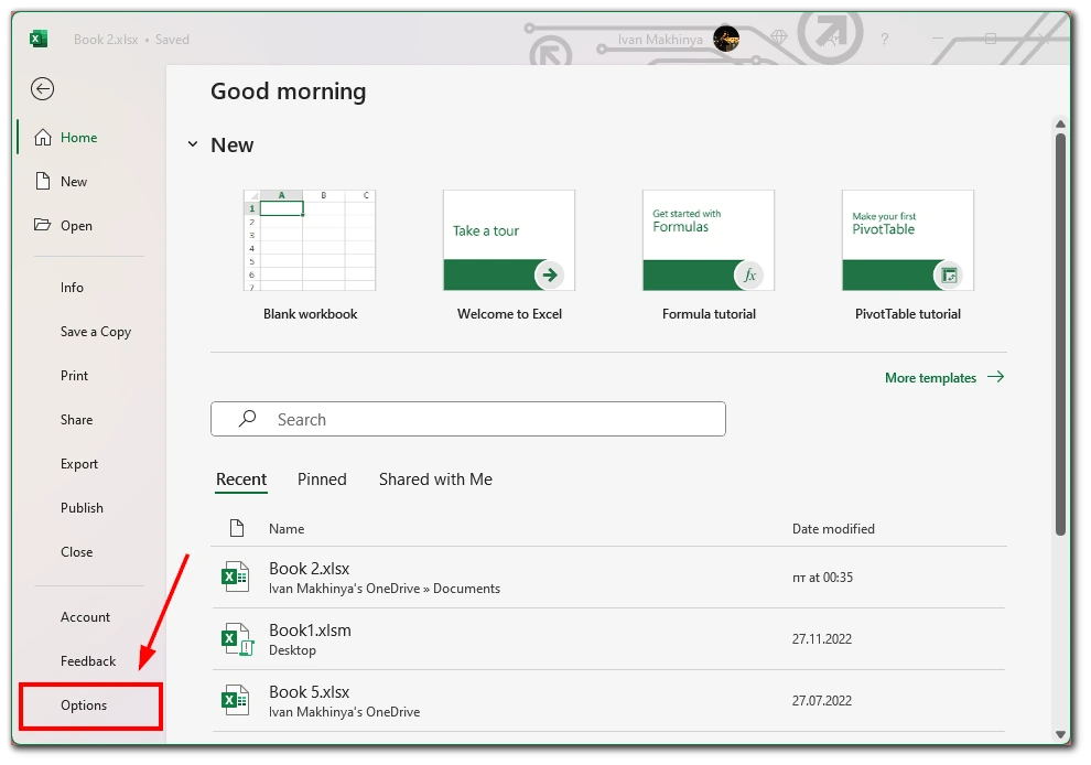
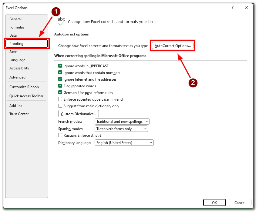
- To set up AutoCorrect, go to the “File” tab, select “Options,” and then choose “Proofing.”
- In the AutoCorrect options, click on the “AutoCorrect Options” button.
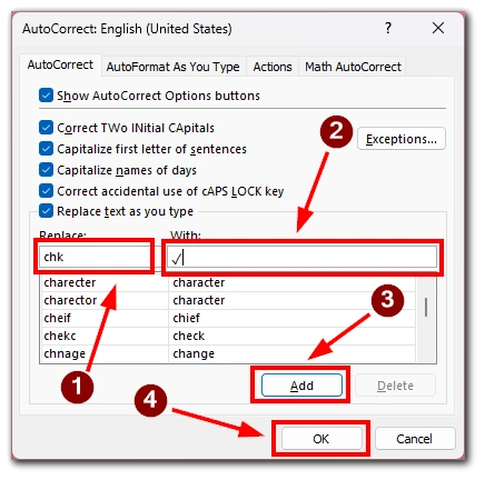
- In the “Replace” field, type a text string (e.g., “chk”) that you want to trigger the replacement.
- In the “With” field, enter the check mark symbol (✓) or copy it from a character map.
- Click “Add,” then “OK” to save the changes.
After that, when you type the defined text string in a cell, Excel automatically replaces it with the check mark symbol. This method is especially useful when you have a large dataset and must frequently insert check marks.
How to insert check marks in Microsoft Excel using Formulas
Excel’s formulas provide a dynamic way to insert check marks based on specific conditions or criteria. One approach is to use the IF function in combination with the CHAR function to display a check mark when a condition is met.
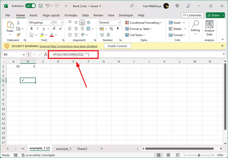
For example, you can use the formula “=IF(A1>50;CHAR(252); " ")” to insert a check mark (☑) in the cell if the value in cell A1 is greater than 50. Adjust the formula and condition based on your specific requirements. This method allows you to automate the insertion of check marks based on the data in your spreadsheet, making it ideal for large datasets or situations where the check marks need to be updated dynamically.
How to insert check marks in Microsoft Excel using Webdings Font
Another method to insert a checkmark in Excel is by utilizing the Wingdings or Webdings font. These fonts contain a variety of symbols, including check marks.
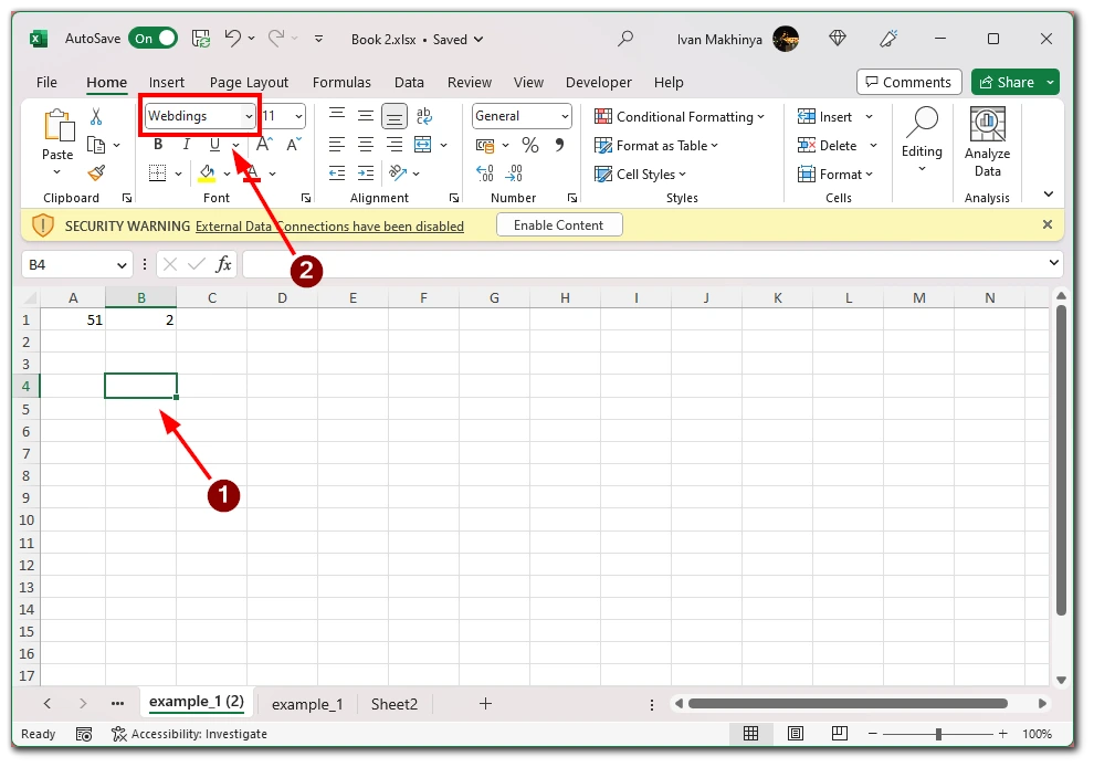
- First, select the cell where you want to insert the check mark.
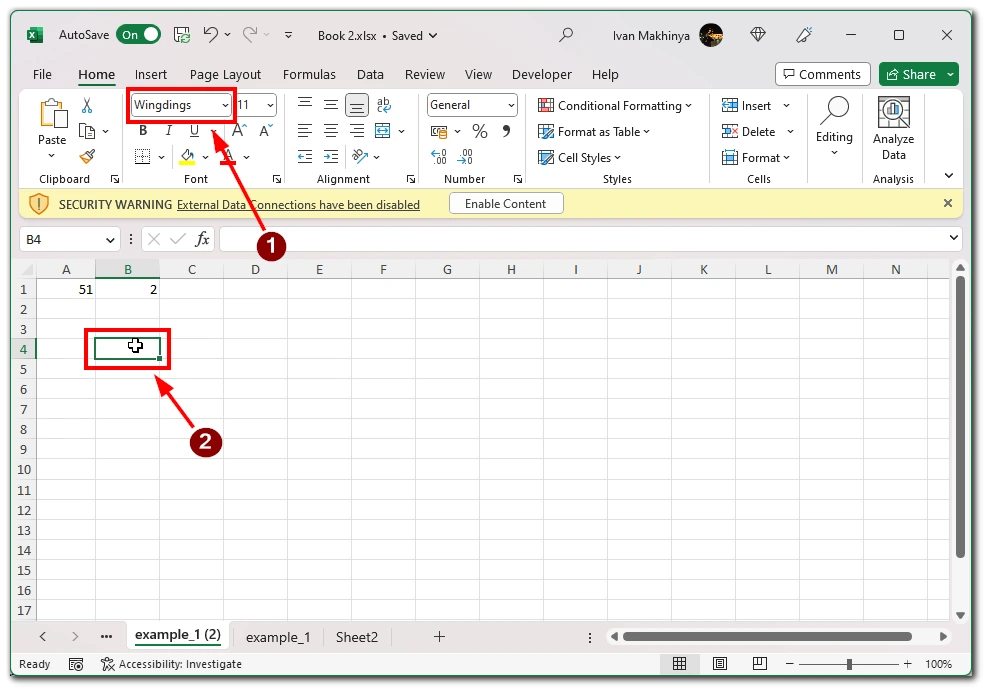
- Then, change the font to Webdings from the font drop-down menu. Next, type the corresponding letter for the check mark symbol. For example, for Webdings, you can use “a” for a check mark (✔).
- Once you type the letter, the corresponding check mark symbol will appear in the cell. This method provides flexibility in choosing different styles of check marks and can be useful if you prefer a specific design.
How to insert check marks in Microsoft Excel using the keyboard shortcut
Another way to tick a box in Microsoft Excel is to use a special combination of keys on your keyboard. However, this method is only available to those who have a Numpad on their keyboard. To insert check marks in Microsoft Excel using a keyboard shortcut, you can follow these steps:
- Select the cell where you want to insert the check mark or navigate to the desired cell using the arrow keys.
- Ensure the font in the cell is set to a font that supports check mark symbols. A commonly used font for check marks is Wingdings.
- Press the “Num Lock” key on your keyboard to activate the numeric keypad if it is not already active.
- Hold down the “Alt” key on your keyboard.
- While holding down the “Alt” key, use the numeric keypad to enter the following code for check marks:
- For a check mark (✓): Press “Alt” + “0252”
- For a boxed check mark (☑): Press “Alt” + “0254”
- Release the “Alt” key. The check mark symbol should appear in the selected cell.
It’s important to note that the keyboard shortcut for check marks may vary depending on the keyboard layout and language settings. The above instructions are based on the standard U.S. keyboard layout.
If the check mark does not appear after entering the keyboard shortcut, double-check the font settings of the cell. Ensure that the font is set to a compatible font like Wingdings or Webdings. If necessary, change the font of the cell to one of these options and try the keyboard shortcut again.
In Microsoft Excel, the ability to insert check marks can greatly enhance the visual representation of your data and improve its readability. Depending on your specific requirements and workflow, you can choose the method that best suits your needs. By mastering these techniques, you can effectively communicate information, track progress, and streamline your Excel spreadsheets with ease.


