

Google Sheets is a really powerful spreadsheet tool because it has all the great formulas. When you enter a formula into a cell in Google Sheets and press the Enter key, Google Sheets instantly calculates the result of the formula and shows the result in the cell. But sometimes you may not want to show the result of the formula, but instead, show the formula itself.
Doing this is easy enough. All you have to do is use the View option to toggle all cells. That way you can display the formula in the cell. This is useful when you need to switch between the two options to check all formulas, but it’s not appropriate for all use cases.
How to show formulas in every Google Sheets cell
It is much more convenient to have all cells at once that display formulas instead of specific numbers. This helps you better understand how your table is structured and which cells may be associated with a potential error. So if you want to do so, you need to follow these instructions:
- Open your spreadsheet and click on the “View” option located in the toolbar.
- Then select “Show” and click “Formulas” to switch this option on.
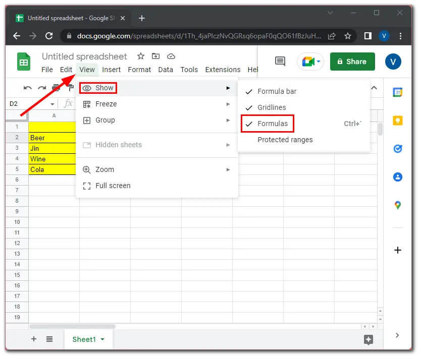
- You can also use the “Ctrl + `” key combination.
- Moreover, you can just double-click on your cell and you will see a formula.
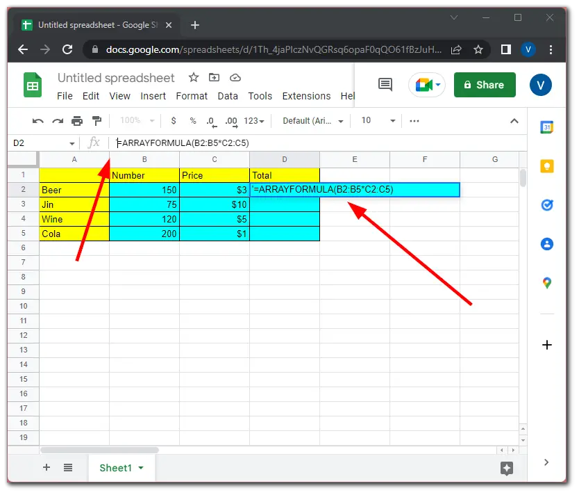
Once you have completed these steps, you will see all formulas showing instead of values in the appropriate cells of your Google Sheets document. Keep in mind that this feature will only show formulas. To hide cells, you need to use other tools. Of course, to hide formulas and return values, you just need to repeat the same steps and uncheck the “Formulas” option.
How to show formulas in one Google Sheets cell
You can also show the formula in a particular cell. Sometimes this can be more convenient, especially if you think the problem is in it. To go this way, just do the following:
- First of all, open your spreadsheet and select the cell with the formula.
- Then put an ‘ in front of the formula in the formula editing field.
All formulas preceded by a single quote will appear on top of the numbers in the cells. You can apply this method to any formula in Google Sheets. The main thing you need to understand is that this sign must come before the equal sign, i.e. before the beginning of the formula itself.
How to hide formulas in Google Sheets using protected tables and ranges
You can use special sheet protection that allows you to prevent other users from editing formulas in locked cells. The following steps will allow you to protect the entire range of cells so that no one can edit the formulas they contain.
- Select the range of cells that contain the formulas you want to hide.
- Click “Data” in the toolbar and select the “Protected sheets and ranges” option.
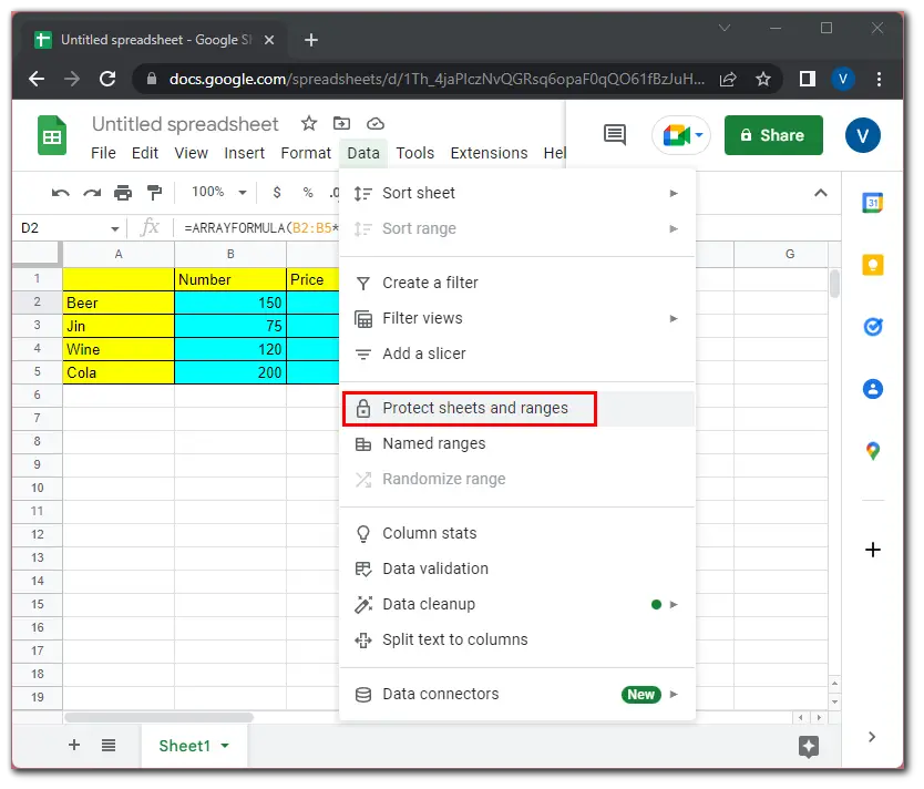
- After that, select “Add a sheet or range” from the pop-up side menu.
- You can add a description and click on the “Set permissions” button.
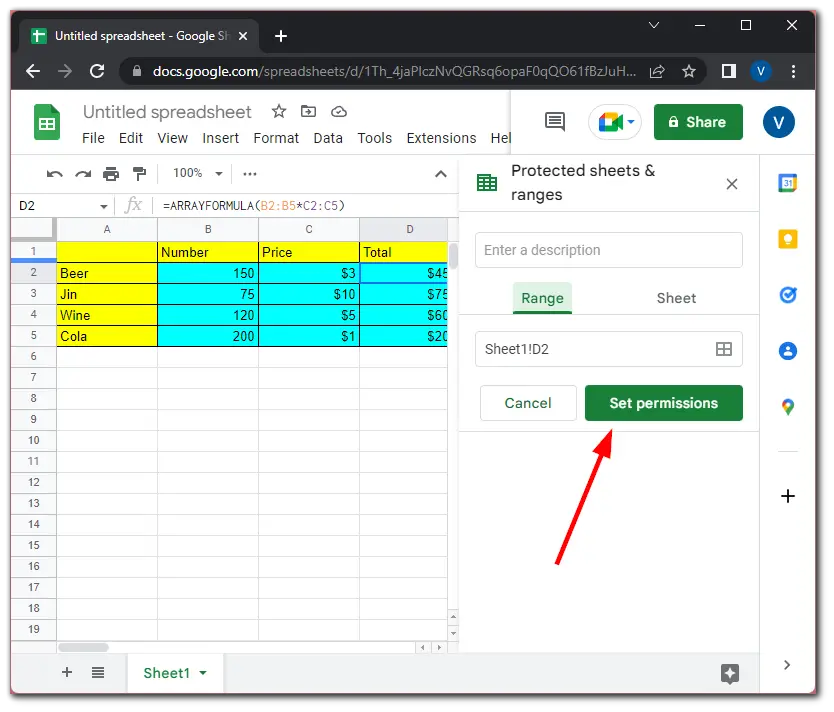
- Finally, in the pop-up window select “Only you” and click “Done”.
This process works to protect individual cells, a range of cells, or the entire sheet.
Read Also:
- How to turn on dark mode in Google Sheets
- How to use the slicer in Google Sheets
- How to create a link to a cell in Google Sheets
How to adjust the color of numbers less than 0 in Google Sheets
If you want to specify all cells where the value can be less than zero, you can use a special rule. This will be especially useful when you need to trace minus when calculating finances. You can use formatting to do so:
- Go to your spreadsheet and click “Format” in the toolbar.
- After that, select “Conditional Formatting”.
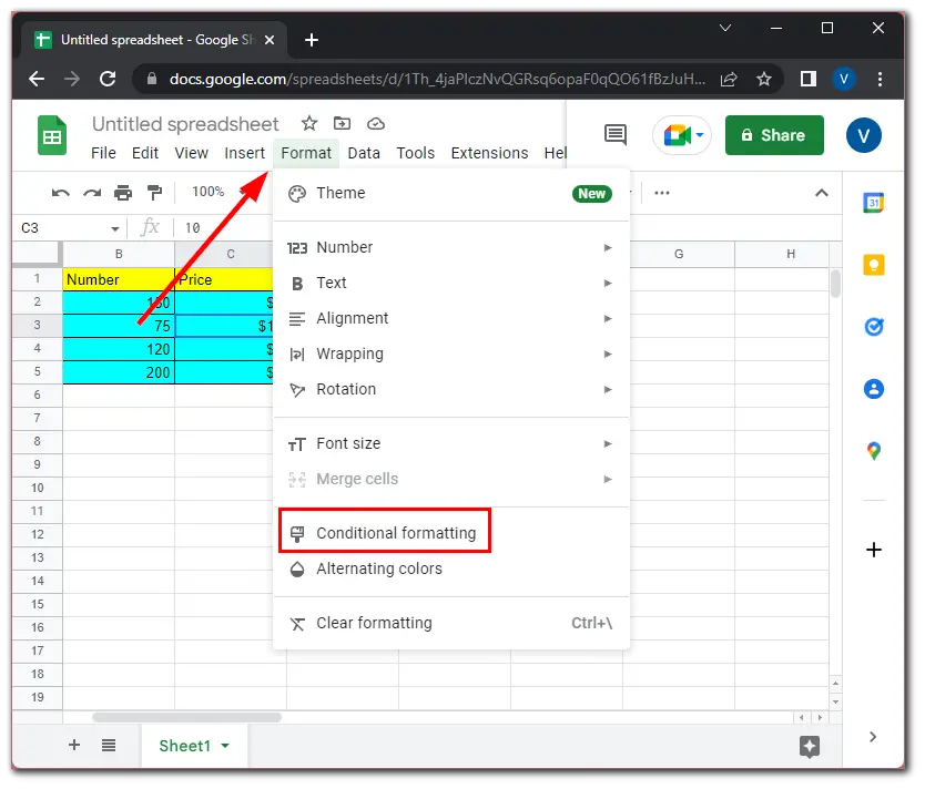
- From the pop-up side menu, select the area to which you want to apply this rule.
- Then select “Less than” from the “Format rules” list.
- In the “Value or formula” field, type 0.
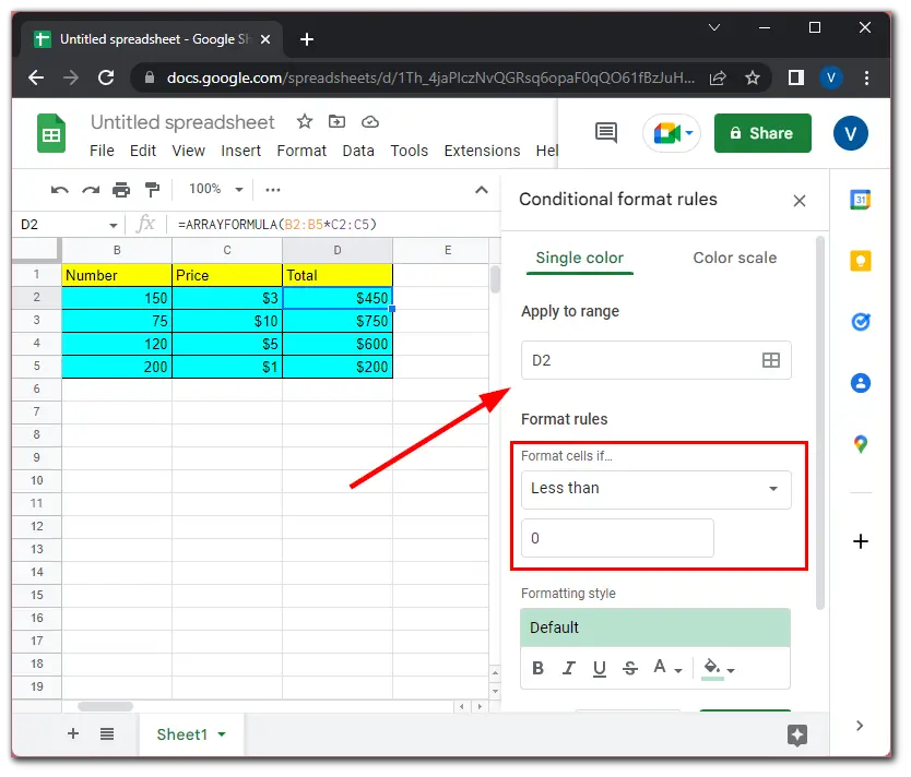
- On the toolbar, select the fill color for the cells that will have a negative value.
- Finally, click “Done”.
Once this is done, the rule will be applied and all cells matching your rule will be filled with the desired color. There are quite a few different conditions that you can apply to your table to highlight the elements you want without having to parse the table manually.


