Slicer is a really handy feature of Google Sheets. It extends the capabilities of crosstabs and summary charts in Google Sheets. And using the slicer is easy enough.

What do you need to use the slicer in Google Sheets

Slider is a Google Spreadsheet tool that lets you quickly and easily filter tables, spreadsheets, and charts with the click of a button. They float above your grid and aren’t attached to any cell, so you can easily move them around the window, align them, and place them however you like.

The slider is called that because it slices through your data, like a filter, to give you customized data analytics. However, it’s better than a filter because it’s much more attractive and user-friendly.

With Slicer, you can analyze data in a much more interactive way. You can create really stunning interactive reports and dashboards right on your Google Sheets worksheet. In fact, once you get the hang of using slicers, you’ll never want to go back to using regular filters again.

Well, here’s how to use the slicer in Google Sheets.

How to create a slicer in Google Sheets

If you want to add the slicer to your Google Sheets document, you have to follow these steps:

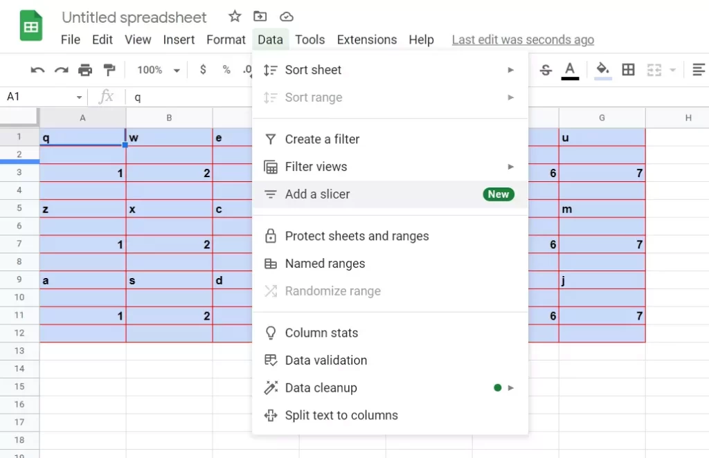
• First of all, choose the chart or table to which you want to apply the slicer.
• Then, click on the “Data” tab and select “Add a slicer”.

• You will see a slicer that looks like a floating toolbar. You can move it to any location on the sheet.
• After that, select the column to filter in the sidebar that appears. If you don’t see the sidebar, double-click “Slicer” to open it.

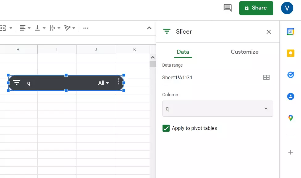
• You should see the column labels for the data you used in the “Column” drop-down list. Select one of them and it will appear in the slice.
• Click on the filter icon or the drop-down arrow on the slice to apply a filter to that column.
  • You will see that you can filter by condition, such as text containing a keyword or values greater than a certain amount.
  • You can also filter by value by deselecting the values you don’t want and leaving the ones you do want highlighted.
• Click “OK” to apply the filter and you will see your data and the chart or table update immediately. You can also see the number of filtered items on the slider itself.

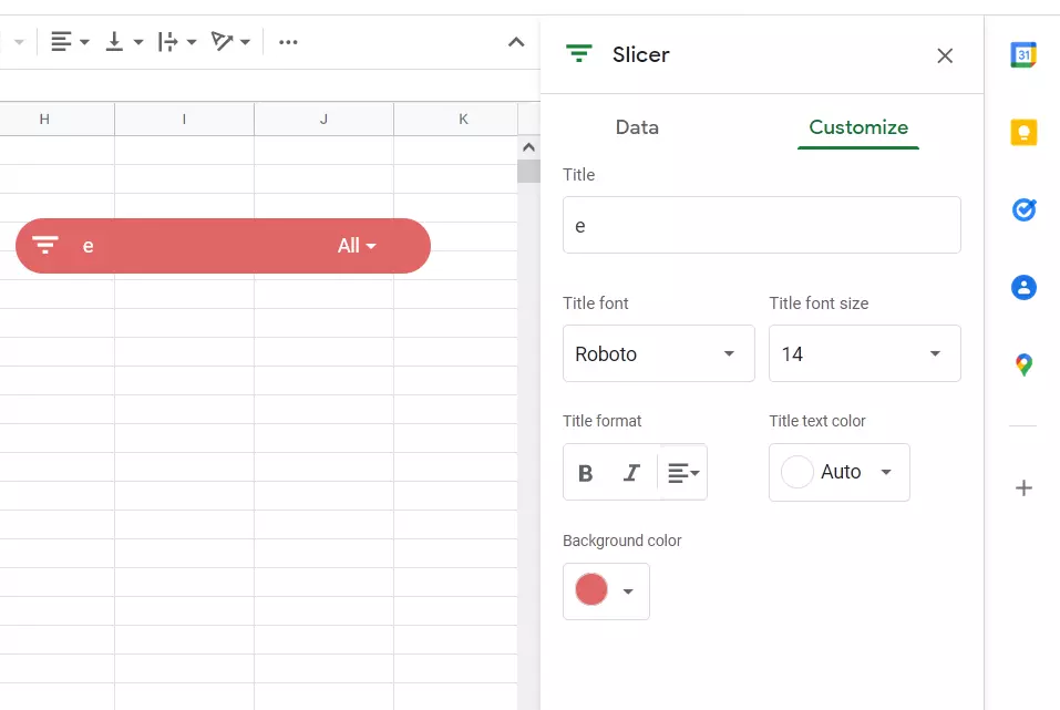
How to customize the slicer in Google Sheets

If you want to change the data set, filter column, or appearance of your slicer, you have to follow these steps:

• Select the slicer and click on the “three dots” icon in the upper right corner
• After that, select “Edit Slicer”.

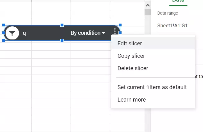
• This opens the “Slicer” sidebar with the “Data” and “Customize” tabs.
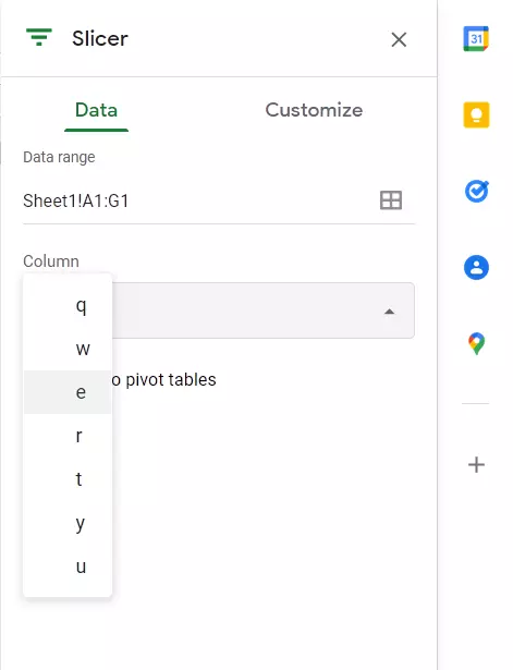
• Use the “Data” tab to adjust the data range or the drop-down column to select another filter column.

• Use the “Customize” tab to change the header, font style, size, format or color, and change the background color.

What are the main terms to use slice in Google Sheets

In conclusion, here are a few important things to keep in mind when using slices in Google Sheets:

• You can connect a slice to more than one table, summary table and/or chart.
• You can only have one slice to filter by one column.
• You can apply multiple slices to filter the same data set by different columns.
• The slice applies to all tables and charts on the sheet, as long as they have the same underlying source data.
• Slices are applied only to the active sheet.
• Slices don’t apply to formulas on the sheet.

That’s all you have to know about the slice in Google Sheets.