

If you see that you have a lot of different-sized cells and want to make them the same size, you should know that there is a straightforward method to help you. However, resizing selected or all cells in Google Sheets is impossible. You can only resize columns and rows separately.
In short, you need to highlight particular rows or columns, right-click on them, and select “Resize rows” or “Resize columns.” Moreover, you can even make all columns and rows the same size at once. To do so, you will need to use a shortcut to highlight them all and then resize them.
So now, let’s look at how it works in more detail.
How to make selected rows the same size in Google Sheets
If you want to make only selected rows the same size in your Google Sheets document, follow these steps:
- Use your mouse to highlight rows you want to make the same size.
- Then right-click on them and select Resize rows.
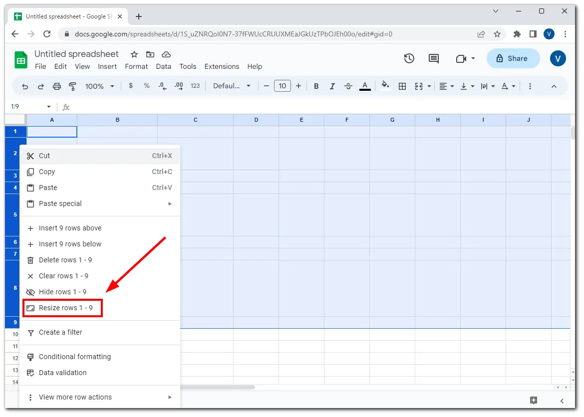
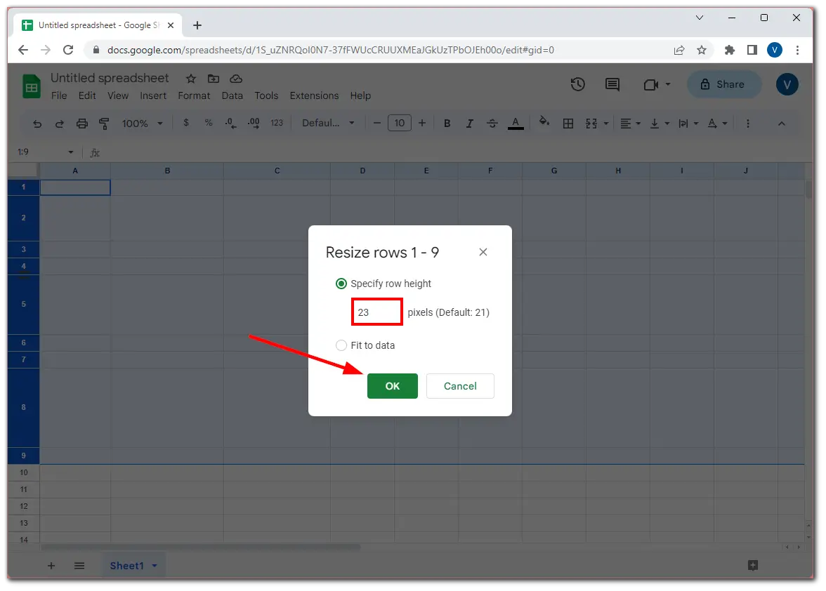
- In the dialog box that appears, enter the desired height for the selected rows and click OK to apply changes.
How to make all rows the same size in Google Sheets
If you want to make all rows the same size in your Google Sheets document, do the following:
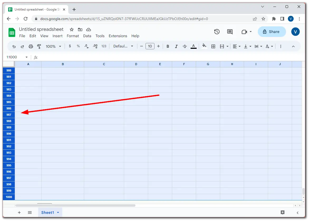
- Highlight the first row and press Ctrl + Shift + Down Arrow.
- You should be taken to the bottom of the spreadsheet, where you will see that all rows are highlighted.
- Now, right-click on one of the highlighted rows and select Resize rows.
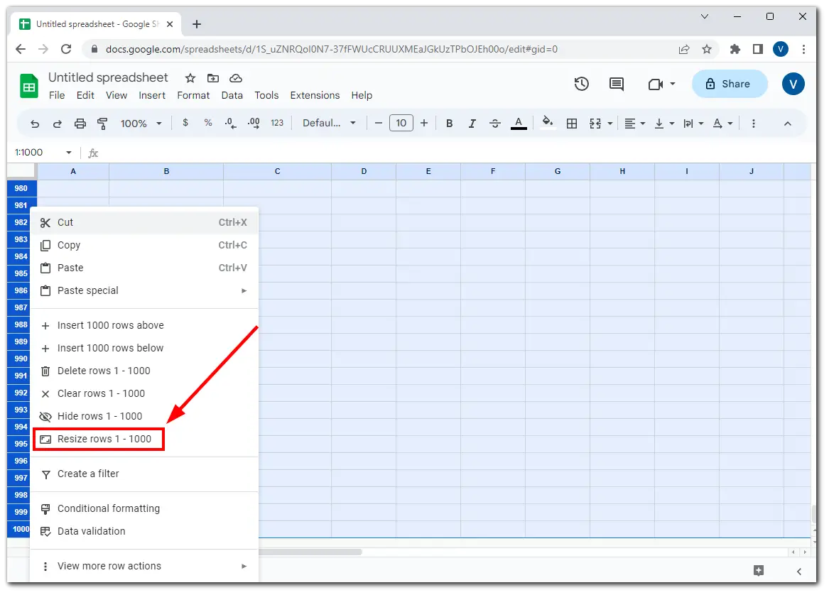
- Enter the desired height and click OK.
For the columns, you can do just the same steps. Let’s look at them below.
How to make selected columns the same size in Google Sheets
Well, if you want to make selected columns the same size in your spreadsheet, you can follow these steps:
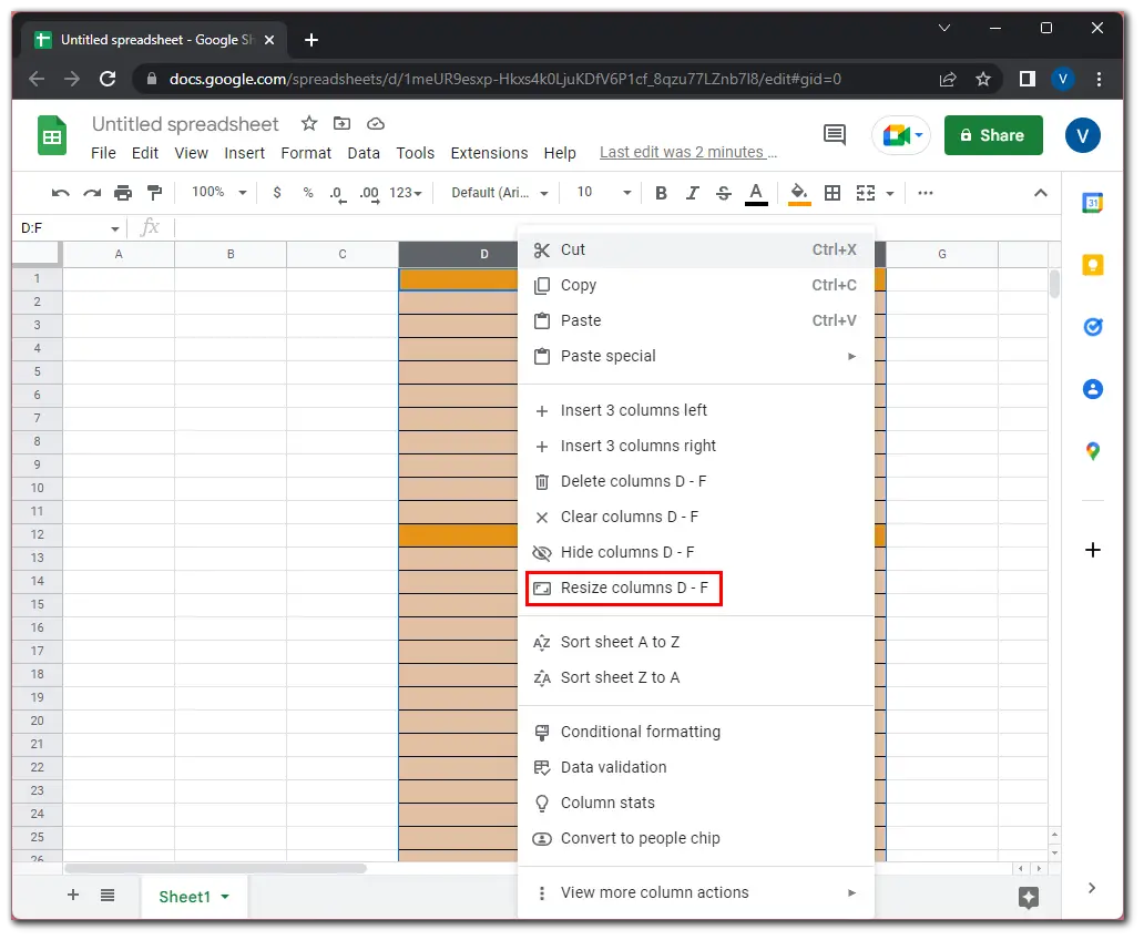
- First, select the columns you want to bring to the same width.
- Then right-click on one of the highlighted columns and select Resize columns.
- When the new dialog box appears, enter the column width. The default column width in Google Sheets is 120 pixels. So let’s enter this number.
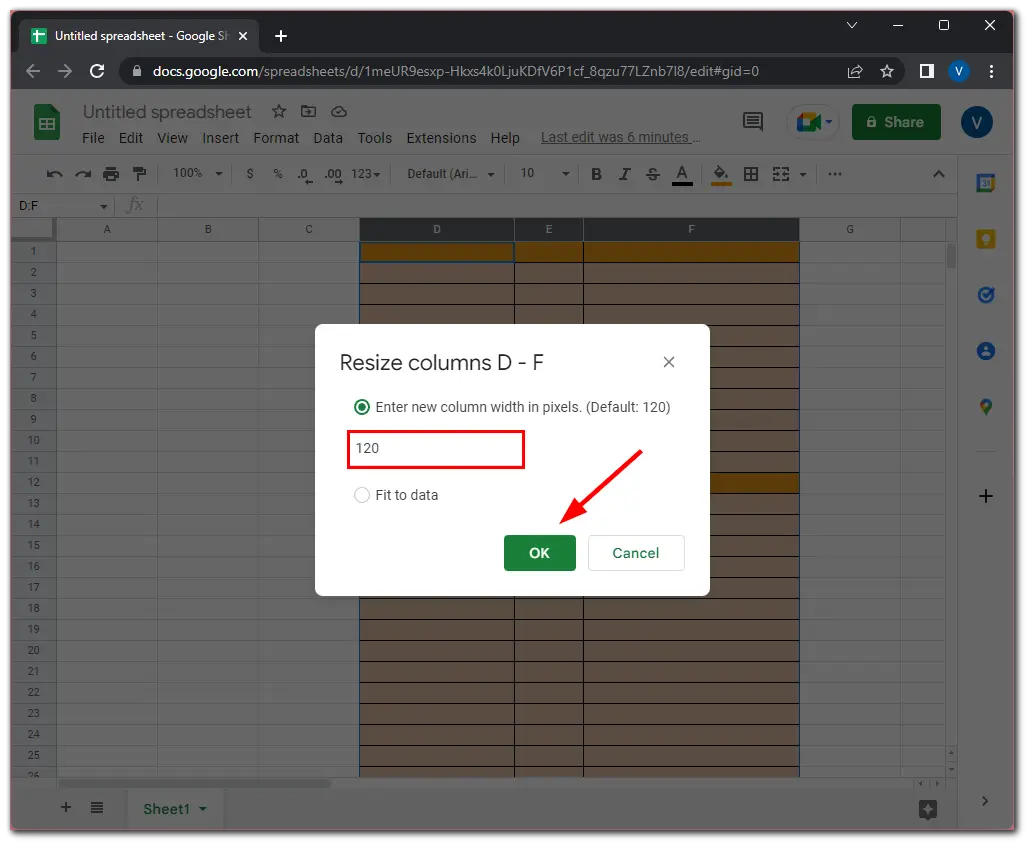
- Finally, click OK to confirm.
How to make all columns the same size in Google Sheets
If you want to make all rows the same size in your Google Sheets document, here’s how:
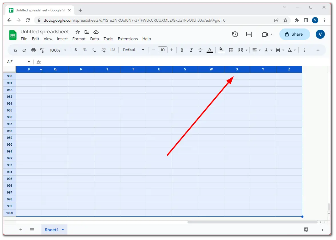
- Highlight the first column and press Ctrl + Shift + Right Arrow.
- You should be taken to the very right of the spreadsheet, where you will see that all columns are highlighted.
- After that, right-click on one of the highlighted columns and select Resize columns.
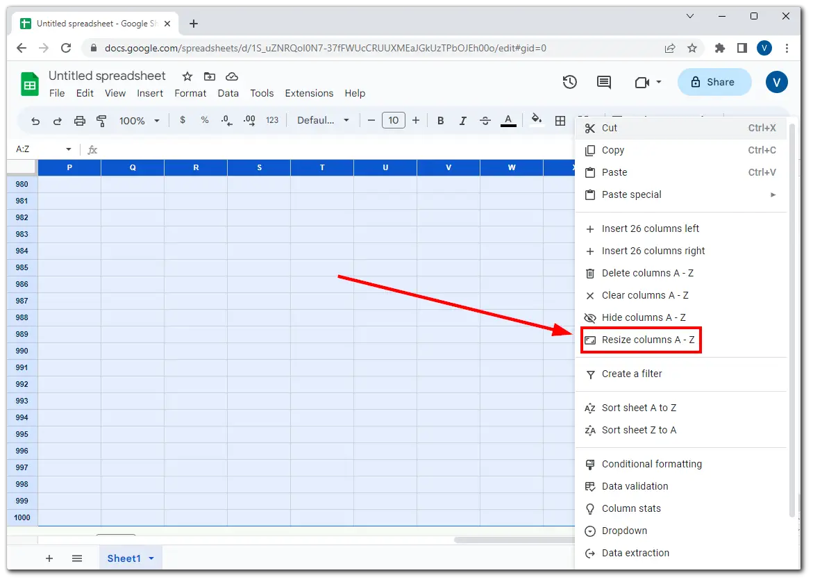
- Enter the desired width and click OK.
That’s it. As you can see, nothing is complicated about making rows and columns the same size in Google Sheets.
Note:
If you choose the “Fit to data” option for rows, Google Sheets adjusts the row height to display the full content of the tallest cell within the selected row. This ensures that all the row’s text, numbers, or other data are visible without any cropping or overlapping.
Similarly, if you apply the “Fit to data” option to columns, Google Sheets resizes the width to accommodate the widest cell content within the selected column. This ensures that all the content in the column is visible without any truncation.
But obviously, this does not guarantee that the columns and rows will all be the same size.
How do I automatically resize cells in Google Sheets?
Have you ever been in a situation where you’re working on a spreadsheet and realize you can’t fit all the data into one cell? You can manually resize the cell, but you may need to see if you can see all of the cell’s content.
Google Tables has two ways to resize cells to fit the content automatically. Here’s how to do it:
Automatically resize cells in a row or column.
Move your cursor to the right of the column header (A, B, C) – the cursor will change to a cross – and double-click the left mouse button (action button). This will automatically resize the column to fit the most extended content in that column.
If the text doesn’t fit your height, move the cursor to the bottom of the header row (1, 2, 3); the cursor will change to a cross and double-click the left mouse button. Your columns will become the size of the most significant content.
To automatically resize multiple columns or rows
Select the columns or rows you want to resize.
Move the cursor to the edge of a selected column/row header.
Double-click and all selected columns/rows are resized to fit the longest/highest content.
Can you make cells the same size on Google Sheets mobile?
Unfortunately, Google Sheets mobile app on iPhone and Android doesn’t provide, for some reason, the selection of multiple rows and columns. You can resize a single column or row, but it’s impossible to get them all to be ideally the same size in this way.
Google Sheets mobile is still primarily focused on viewing and editing spreadsheet data on a small screen, and some advanced formatting features, such as adjusting the size of multiple rows and columns, are not available.
So, for now, the only way to do it is to use the desktop version.


