

Excel is the most popular spreadsheet system in the world. Excel is especially popular with corporate workers. This is because Excel has many tools that help you quickly post different things in your spreadsheet or fill it out. Excel can also work well with other popular Microsoft Office applications and services such as OneDrive virtual storage and Outlook email. One of the tools you should look into is the ability to calculate the probability of an event.
You can use simple formulas like multiplication and division, create a complex equation to calculate probability or use the built-in PROB formula to calculate probability in Excel. Of course, first of all, you need a good table and structure of your data to make PROB work correctly. So before applying it to actual work, I advise you to practice with simple examples and carefully read this article, where I will try to explain everything in detail.
What formulas can you use to calculate probability in Excel?
As I said above, you can calculate probability in two ways: manually and with the usual arithmetic formula and a particular function. Let me briefly explain how to quickly calculate the probability manually and then explain exactly how the formula works for more complex calculations. If specifically interested in the PROB formula, scroll to the next heading.
Let’s first understand how probability works in general. Probability is how much chance there is of this or that event happening. In the case of numbers and tables, it is the probability that this or that number will be chosen if you choose random numbers from a table. You can use a more straightforward method if you have a table with two columns.
To do this, you need to calculate how many times your table repeats the number for which you need to calculate the probability and divide this number by the total number of numbers in your table. As you can see, this is pretty simple. For example, if you have 20 numbers in your table and five times the number you need to calculate the probability, then you need to use the formula “=5/20”. The probability of such a number falling out would be about 25%.
How to use the PROB function in Excel
The PROB function calculates the probability of an event or several events. It is helpful if you know the probability of each event, but you need to calculate the probability of two events occurring in parallel. For example, if you know that the probability of your workshop being attended by ten people is 20% and that 20 people are coming is 15%. The PROB function helps you to calculate the probability of having between 10 and 20 people attend. The syntax of this function is:
= PROB(x_range, prob_range, [lower_limit], [upper_limit])
Let’s take apart each element in this example, and I will explain what it is for:
- x_range is numbers that are connected with probabilities. Roughly speaking, these are the numbers whose probability you need to calculate.
- Prob_range is the probability for each number that is involved in your example. The sum of the probability column should always reach precisely 1 or 100%.
- Lower_limit (optional) is the minimum limit among the numbers you need to find. It is optional.
- Upper_limit (optional) is the maximum limit of the numbers you have to find. This is optional.
The PROB function looks a bit complicated and confusing at first sight. It is helpful in quite a few situations. I recommend you to read the next section, where I will show you how to correctly calculate probabilities in an Excel spreadsheet using the PROB function and the usual arithmetic formulas to determine the probability.
An example of probability functions in Excel
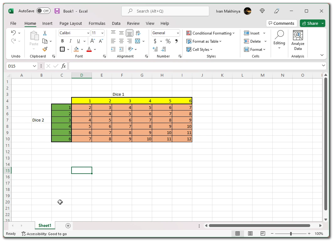
Let’s look at a simple example with two cubes. I’ll show you how to calculate the probability that you will roll one specific number from 2 to 12. To begin, we need to make a table that lists all possible combinations of the numbers from the two dice. This table will look something like this:
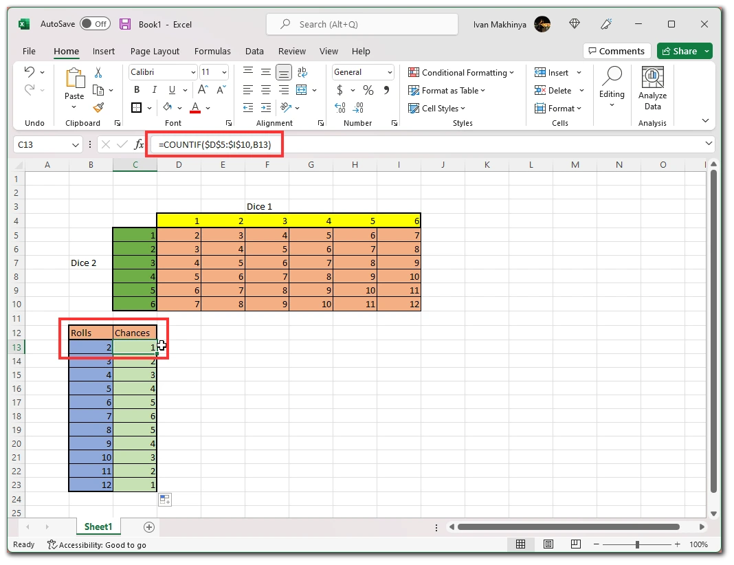
After that, we need to calculate the odds of each number falling out. For example, we have only one chance of getting two or only two chances of getting three. You do this with the simple formula.”=COUNTIF([Table_Range], [digit you want]).” In practice, this formula would look something like this:
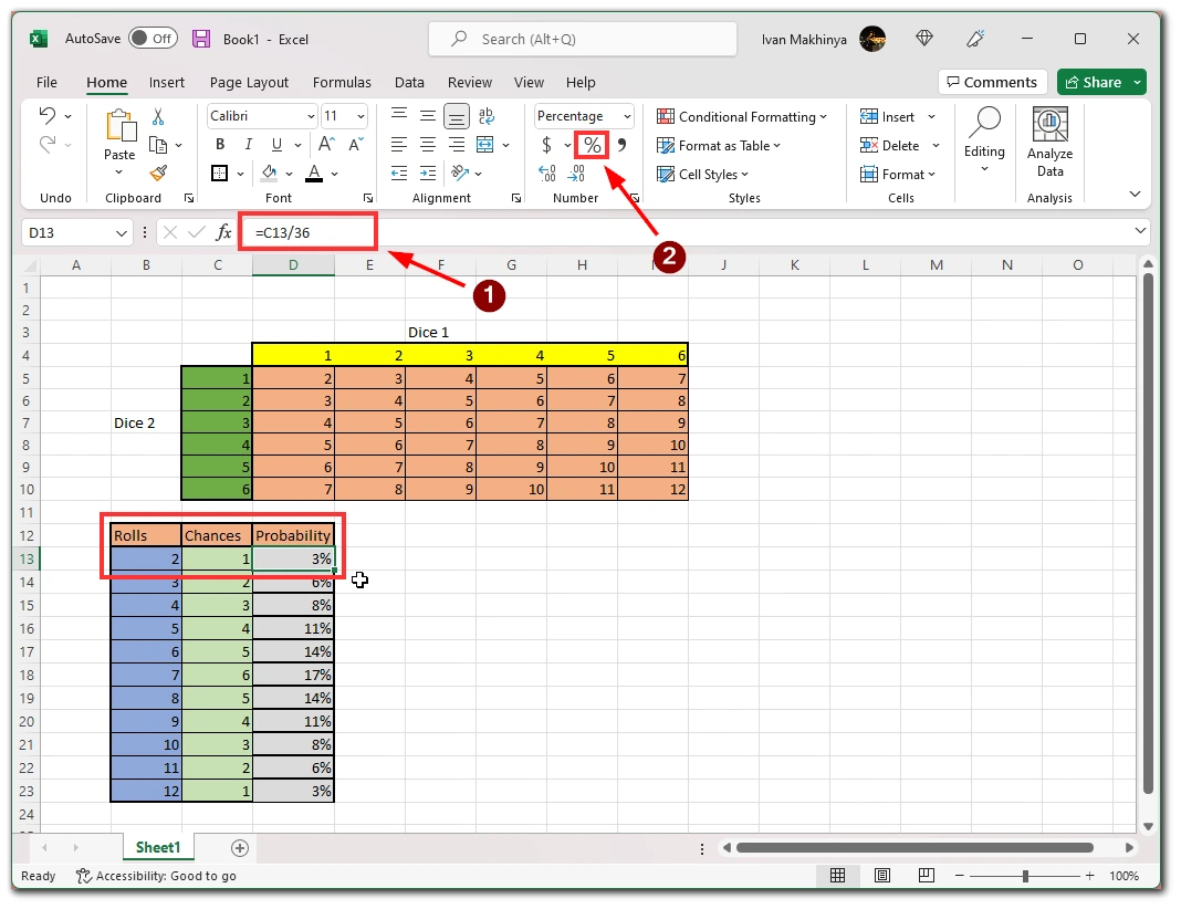
Next, we need to calculate the probability of falling out for each digit that might fall out. To do this, you need to divide the number of chances to fall out by the maximum number of possible choices. In this case, that would be 36:
Afterward, you will get a column with the probabilities of each number falling out on your dice. We can use the PROB function to determine which number has a better chance than 5. It will look like =PROB([Rolls_Range], [Probabilities_range],[Lower_limit],[Upper_limit]). In our example, it looks like this:
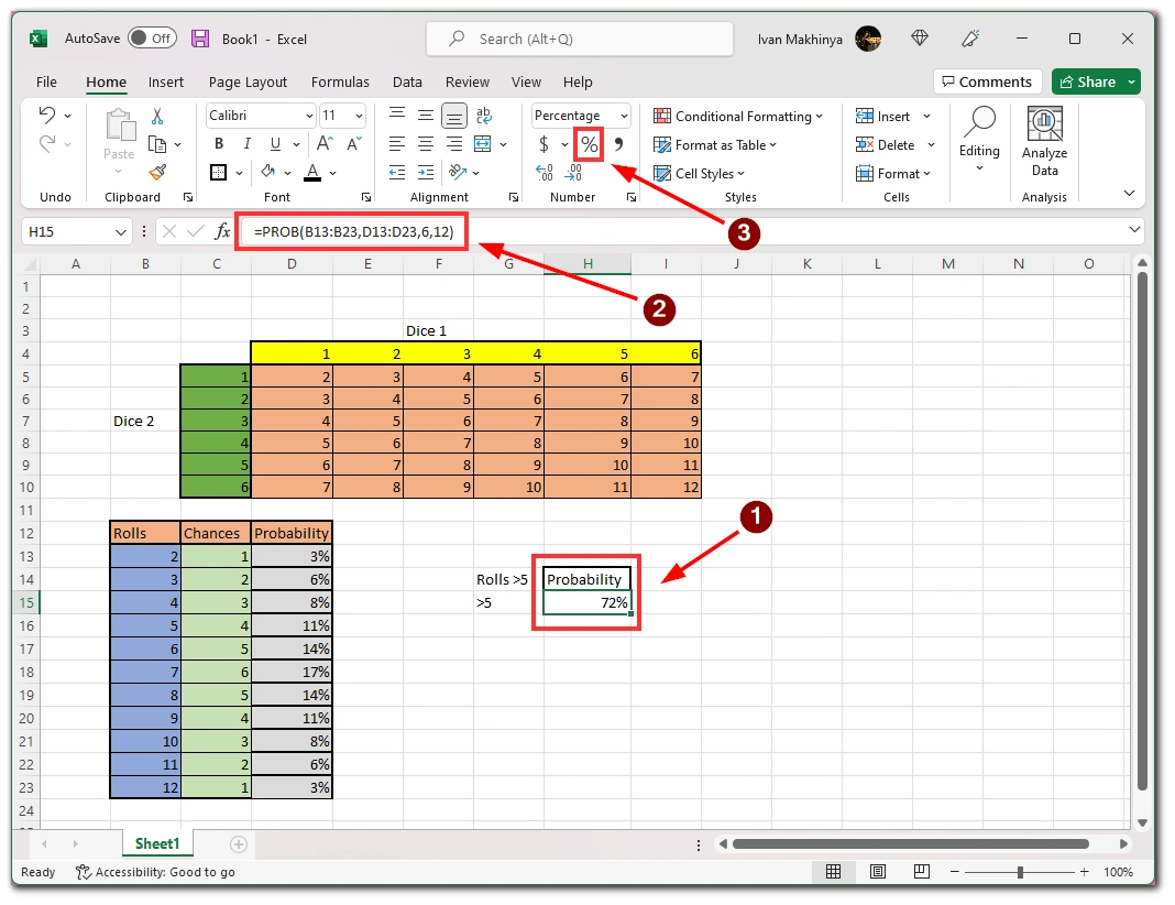
So we got that the probability of a number greater than 5 is 75%. You can use this method to calculate probabilities from any table you need. Try experimenting with this or other simple examples to see exactly how it works.


