

Strikethrough text in Word is really easy, you just need to press the strikethrough button in formatting options, and voila, the text is crossed out! But things don’t work the same way in Excel and the strikethrough button isn’t easy to find. It’s in the same place in Excel Online, but it isn’t here in the desktop Excel app.
There’s a strikethrough option in Excel as well, but it’s hidden away, maybe because it isn’t so popular in this app.
Here are different ways you can use to cross out text in Excel.
How to cross out text in Excel manually
If you need to strikethrough text only sometimes and don’t want to use any shortcuts or other more complicated ways, you can cross it out manually. Here’s how:
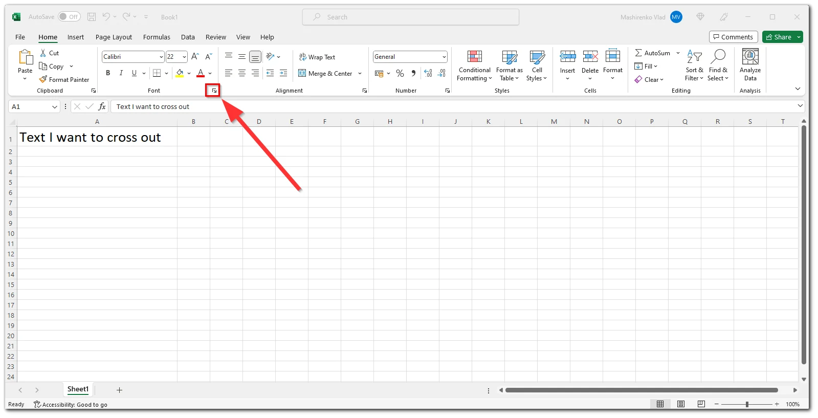
- Select the text you want to strikethrough.
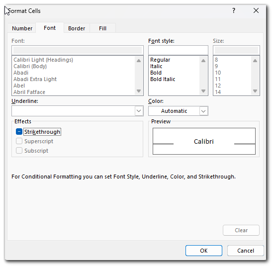
- In the Font Options section, click on the arrow in the bottom-right corner.
- Here, select Strikethrough among the list of Effects.
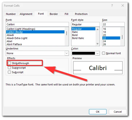
- Click OK and your text would be crossed out.

As you see, it takes literally 3 clicks, but if you need to strikethrough quite often, that’s inconvenient, as to use Excel like a pro you need to automate your actions with shortcuts.
How to strikethrough text on Excel with a shortcut
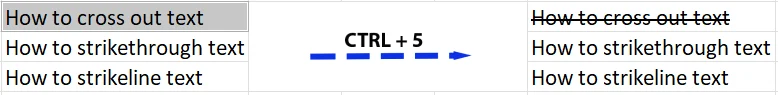
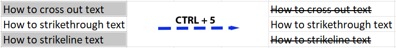
Here’s a hotkey combination to cross the text out, you just need to press CTRL+5. It works for the cell as a whole, for a couple of cells, or for just some text inside the cell (for this you need to double-press on it to enter cell edit mode).
You can also press and hold CTRL to strikethrough cells that aren’t placed next to each other. Just hold CTRL and press 5 any time you want to cross out the cell.
Here’s how it works with examples.
- PressCTRL+5to strikethrough one cell or cells placed next to each other:
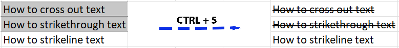
- Press and holdCTRLto strikethrough non-adjacent cells, and press 5 to strikethrough the chosen cells:
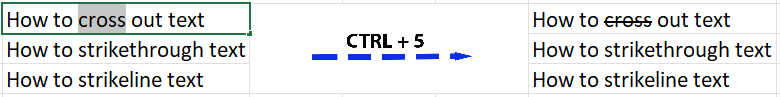
- To strikethrough only part of text inside the cell, double-click the cell to enter edit mode, highlight the part of the text and press CTRL+5:
Okay, now you know how to strikethrough text in Excel via cell format options and using the Ctrl+5 shortcut. But you can also add a strikethrough action to Quick Access Toolbar, so it would look like in Word (in a different place, but still it would be almost the same).
How to add a strikethrough button to Quick Access Toolbar
As I said, this way you will add the button to the Toolbar, it looks the same as in Word. Here’s how:
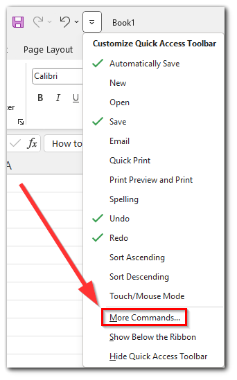
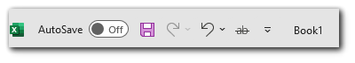
- Tap the arrow near to Toolbar icons (save, undo, redo, etc.) and choose More commands… from the drop-down menu.
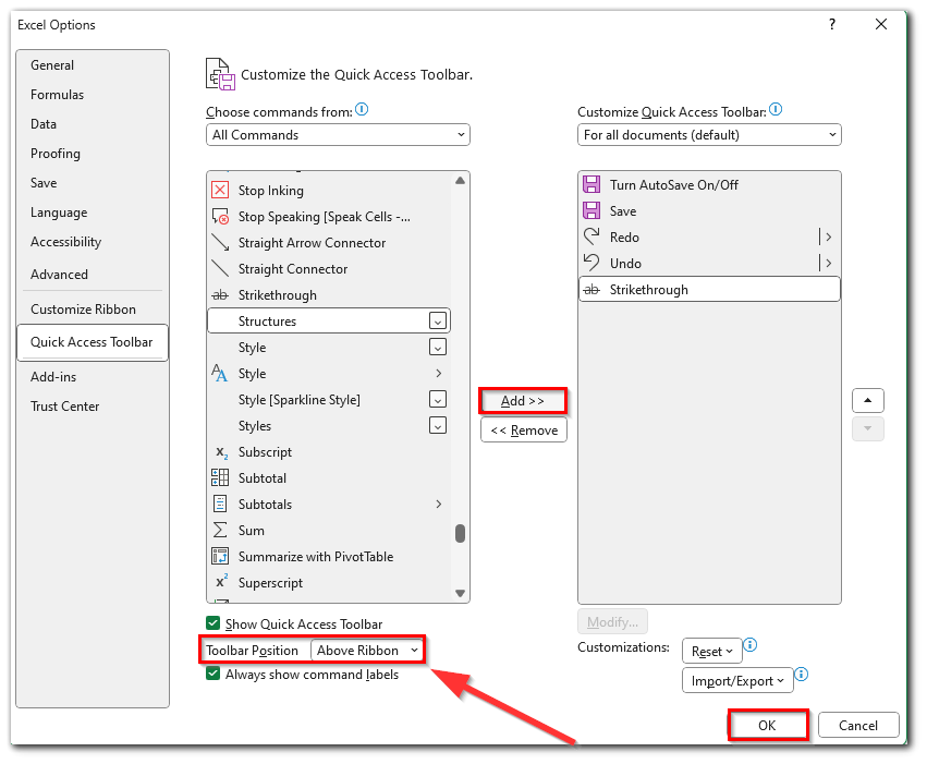
- Here you need to choose All commands and find Strikethrough in the list (yeah, there’s no search, but all commands are listed alphabetically) and then click Add.
- You can also change the Toolbar position and place it below Ribbon (as the arrow indicates on the screen).
- Now, the strikethrough icon would be placed in Quick Access Toolbar and you can use it the same way as in Word.
You can also put a Strikethrough button on the Excel Ribbon. You can use this instead of adding it to Quick Access Toolbar.
How to add a strikethrough button to Ribbon in Excel
I don’t like using Quick Access Toolbar because it’s a place for the most frequently used commands and strikethrough is 100% not in this list. If you think the same, you can consider using ribbon instead. You can add the Strikethrough command here:
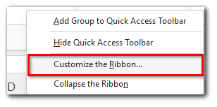
- Right-click on the empty space on the Ribbon and click Customize the Ribbon…
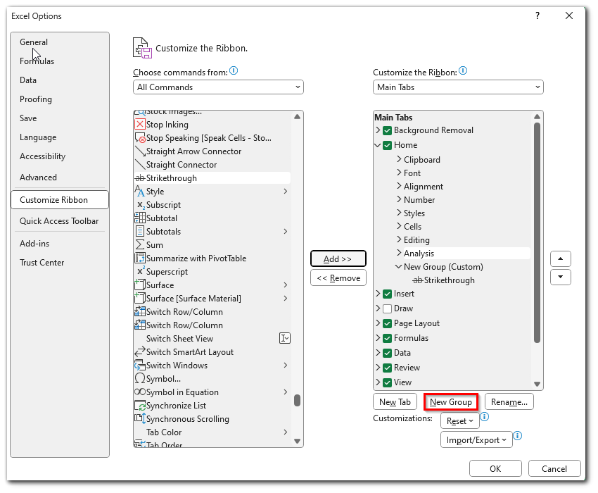
- Select All Commands and find Strikethrough. Don’t forget to create a New Group, because commands should be added to custom groups.
- Now the Strikethrough button would be displayed on the ribbon and you can use it.
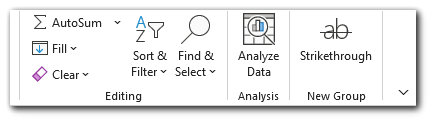
- If you want to move this command on the ribbon, you can do so by using by dragging and dropping your custom group in Customize the Ribbon… window.
How to add Strikethrough to conditional formatting
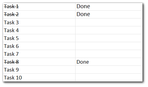
This feature may be useful if you’re using Excel to manage to-do lists or something like that. You can add strikethrough to conditional formatting rules, so the text in the cell would be automatically crossed out when needed. For example, when you provide input “Done”.
Here’s how to set up this:
- Select the cells range you want to apply conditionals for.
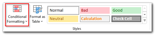
- On the ribbon, click on Conditional Formatting.
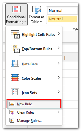
- In the drop-down menu choose New Rule.
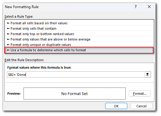
- In the dialogue window, select Use a formula to determine which cells to format and enter the top input cell (like =$B2=”Done”).
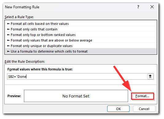
- Now click Format…
- Check the box next to Strikethrough. You can also add some additional formatting, like different text colors.
- Now, when the input is Done, the cells would be crossed out automatically.
You can also add checkboxes and set the conditional formatting to strike text through when they’re TRUE.
How to strikethrough in Excel Online
In Excel Online everything looks like in Word, so you can follow these steps:
- First of all, go to the Home tab.
- Then click on the “Font Settings” option located in the “Font” section.
- After that, you will see the “Strikethrough” option in the appearing list.
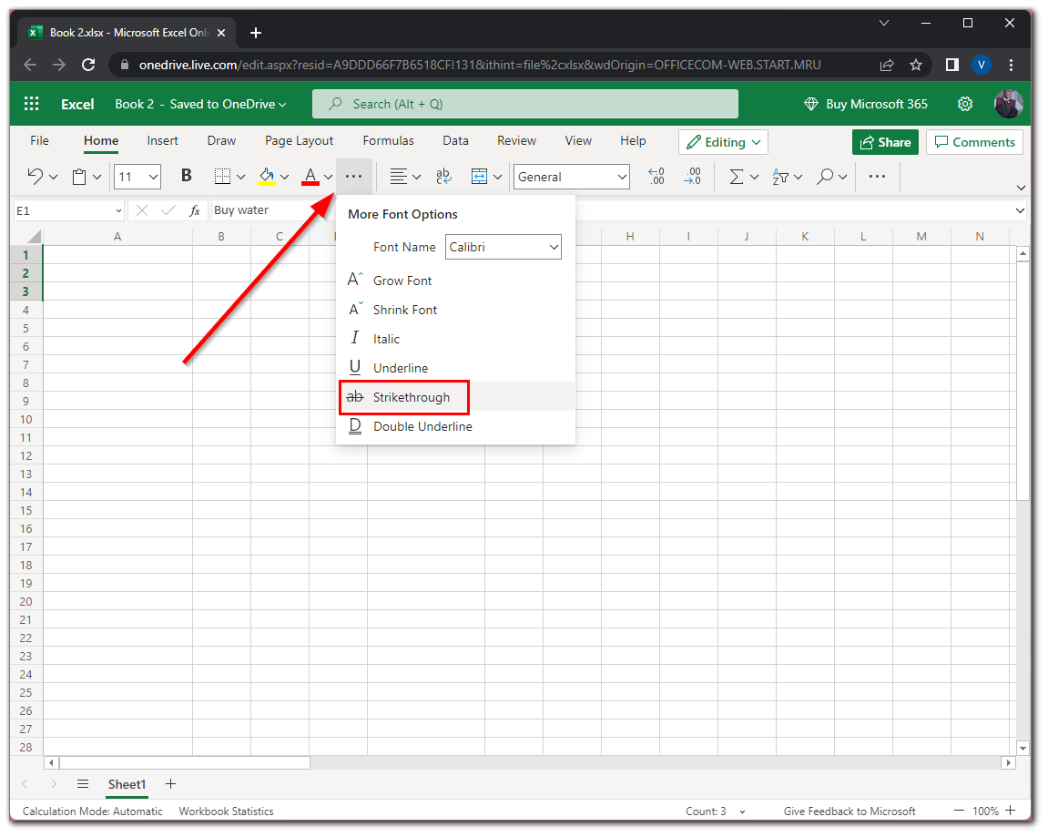
- Finally, select this option and you will see that the items in cells are become crossed out.


how to undo this action?