

The Gantt chart is an easy-to-use and clear tool for displaying current tasks with their reference to real-time. Such a chart allows you to see not only the number of available tasks, but also their priority, volume, and time left to complete them.
Many project managers say that using Gantt charts is their protection against missing deadlines. It’s an opportunity to always see in what order to solve tasks, and not to forget about any to-do. And you don’t always need specialized software to work with this handy tool – a Gantt chart in Google Sheets can be just as handy as its counterpart built in a more specific environment.
Well, here’s how to create a diagram in Google Sheets, how to work with it, and who it will be useful to, we will talk below.
What is a Gantt chart
It’s essentially a type of bar chart, in which each separate column (row) corresponds to a particular task. Depending on its location and size, it illustrates the start and completion times of the corresponding phase. You can place tasks in the Gantt chart both according to the sequence of work to be done and according to their priority.
Consequently, it can be used both in a traditional linear project system, where it’s important to follow the initially set sequence, and it can be used in flexible methodologies that allow editing the list of tasks and their priority.
This type of diagram was originally developed by Henry Gantt to manage the activities and tasks of engineers in an English shipyard. He assembled subordinates’ tasks into separate lists, defined the resources required for them, and the dependence of one task on another. He also calculated the time required to complete each type of task, the labor intensity of each individual task, and the responsibility of one or another employee for completing them.
Then Gantt transferred these results to a diagram chart, relating the stages of work to time – and thus obtained a model that clearly represented the structure of the project, the progress, and the volume of each task in its structure. Subsequently, Gantt charts have changed and modified somewhat, new ways of constructing them have appeared, including through Google Sheets tools – but the basic essence remains unchanged.
How to create a Gantt chart in Google Sheets
If you want to create a Gantt chart in Google Sheets, you have to follow these steps:
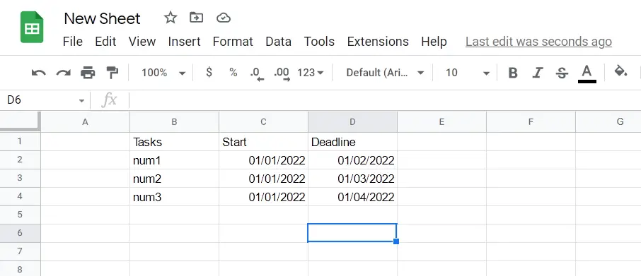
- Create a sheet with a complete list of tasks and their start and deadline dates
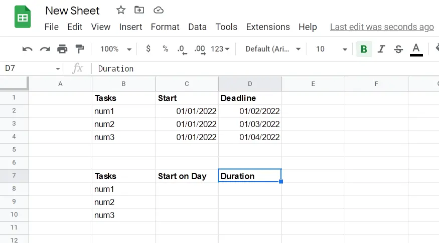
- Then, create a similar sheet on the side or below the previous one that will be used to calculate the graphs in each part of the Gantt chart. The table will have three headings for the Gantt chart: the tasks, the start day, and the duration (in days) of the task.
- After you set up the headers, you need to calculate the start day and duration. The “Tasks” header will be the same as the one above. You can simply copy the cells below it, reference them directly, or rewrite them if you want.
- To calculate “Start on Day”, you need to find the difference between the start date of each task and the start date of the first task. To do this, you must first convert each date to an integer, and then subtract it from the start date of the first task.
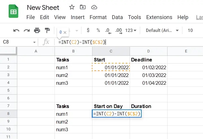
- In a formula, the <FirstTaskStart>will always be an absolute value. Google Sheets uses a dollar sign ($) to “lock” a row or column – or, in our case, both – when referencing a value.
- Thus, when you copy the same formula for subsequent cells, using the dollar sign in this way ensures that it will always refer to the value in C2, which is the beginning of the first task.
- After pressing Enter, click the cell again, and then double-click the small blue square.
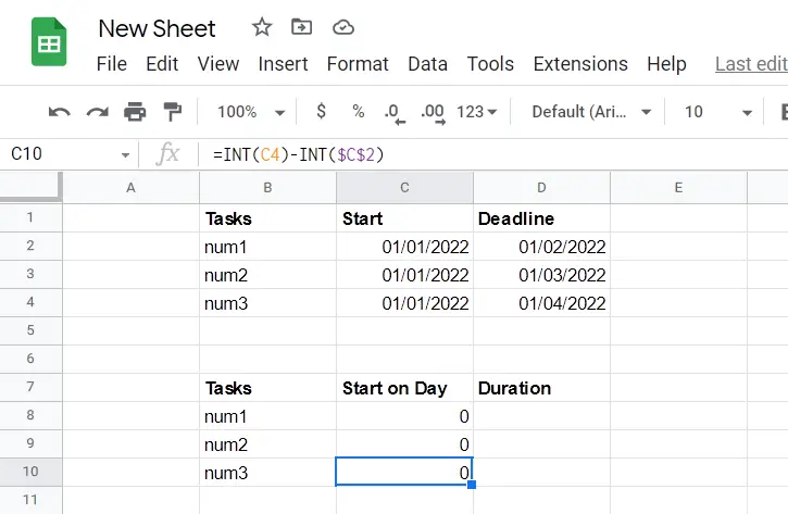
- The sheets will use the same formula – but necessarily referencing the correct cell above – for the cells immediately below them, completing the sequence.
- Now to calculate the duration, you need to determine how long each task will take. This calculation is a bit more complicated, and you can find the difference between several more variables. =(INT(D2)-INT($C$2))-(INT(C2)-INT($C$2))
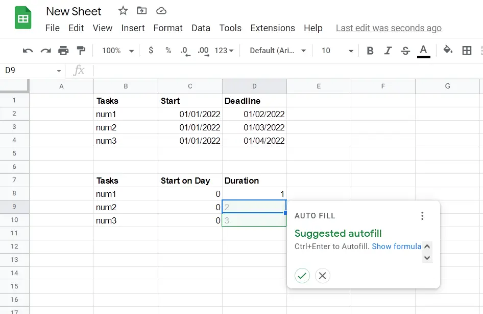
- Just click on the green checkmark to confirm the autofill.
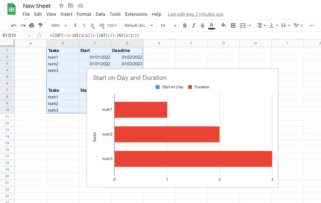
- After that, highlight the entirety of the table and click “Insert”.
- Select “Chart” and voila. The Gannt chart is ready.
As you can see, creating Gantt charts in Google Sheets is quite possible, but you will need to have either reference information or a template on hand, which will still need to be customized and edited later.


